import numpy as np
import matplotlib.pyplot as plt

mean = 1
variance = 1
num_samples = 1000
np.random.seed(1)
samples = np.random.normal(loc=mean, scale=np.sqrt(variance), size=num_samples)
print(samples.shape)(1000,)import numpy as np
import matplotlib.pyplot as plt
mean = 1
variance = 1
num_samples = 1000
np.random.seed(1)
samples = np.random.normal(loc=mean, scale=np.sqrt(variance), size=num_samples)
print(samples.shape)(1000,)Let’s analyze the samples
# First 5 elements
print(samples[:5])
[ 2.62434536 0.38824359 0.47182825 -0.07296862 1.86540763]Visualizing the random samples
plt.hist(samples,bins=30)
plt.title("Histogram of samples with mean and variance 1")
plt.show()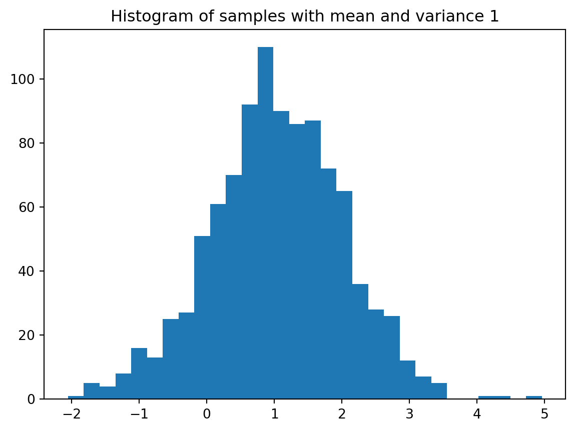
The likelihood for the normal distribution is given by,
\[ L(\mu,\sigma^2;x_1,x_2,....,x_n) = \prod_{j=1}^n f(x_j;\mu,\sigma^2) \]
where f, is the probability density function which in this case is the univariate normal distribution given by,
\[ f(x,\mu,\sigma^2) = \frac{1}{\sqrt{2\pi\sigma^2}} e^\frac{-(x-\mu)^2}{2\sigma^2} \]
The likelihood of a distribution with given mean and variance is the product of value of PDF at all sample points with given mean and variance. Likelihood gives us a fair estimate or probablity as to how well the distribution is fitting the data for given parameters (mean and variance in case of normal distributon). So the probability that the normal distribution with given mean and variance will fit the samples is a product of the value of the pdf at each sample point as all these events are independant events. Hence, plotting the likelihood or the log-likelihood as function of parameters (in this case mean and variance) can give us an estimate as to which values of parameters are needed to best fit the data.
Likelihoods are generally products of many numbers and products are not numerically stable. Hence, log-likelihood is calculated to make computations less expensive and simpler.
Taking log on both sides,
\[ \begin{equation} \begin{split} l(\mu,\sigma^2;x_1,x_2,...,x_n) & = ln(L(\mu,\sigma^2;x_1,x_2,...,x_n)) \\ & = ln((2\pi\sigma^2)^\frac{-n}{2} e^\frac{-\Sigma_{j=1}^n (x_j-\mu)^2}{2\sigma^2})\\ & = ln(2\pi\sigma^2)^\frac{-n}{2}+ln(e^\frac{-\Sigma_{j=1}^n (x_j-\mu)^2}{2\sigma^2}))\\ &= \frac{-n}{2}ln(2\pi\sigma^2)-\Sigma_{j=1}^n \frac{(x_j-\mu)^2}{2\sigma^2} \end{split} \end{equation} \]
The above equation can be used to compute the log-likelihood.
log_likelihoods = []
for mean in np.linspace(0, 2, 100):
    for var in np.linspace(0.1, 2, 100):
        log_likelihood = np.sum(-0.5 * np.log(2 * np.pi * var) - ((samples - mean) ** 2) / (2 * var))
        log_likelihoods.append((mean, var, log_likelihood))

log_likelihoods = np.array(log_likelihoods)
print(log_likelihoods.shape)
(10000, 3)The log_likelihoods array is a 2D-array with mean values in the first column, variance values in the second column and likelihood values in the third column. Let’s look at the first 5 rows of the array.
log_likelihoods[:5]array([[ 0.00000000e+00, 1.00000000e-01, -9.97514834e+03],
[ 0.00000000e+00, 1.19191919e-01, -8.41934984e+03],
[ 0.00000000e+00, 1.38383838e-01, -7.30630086e+03],
[ 0.00000000e+00, 1.57575758e-01, -6.47285210e+03],
[ 0.00000000e+00, 1.76767677e-01, -5.82700895e+03]])A 3D plot of how log-likelihood varies with mean and variance can be seen below.
fig = plt.figure()
ax = plt.axes(projection='3d')
ax.plot3D(log_likelihoods[:,0],log_likelihoods[:,1],log_likelihoods[:,2],color='green')
ax.set_title("Log-likelihood of normal distribution as a function of mean and variance")
ax.set_xlabel("Mean")
ax.set_ylabel("Variance")
ax.set_zlabel("Log-likelihood")
plt.show()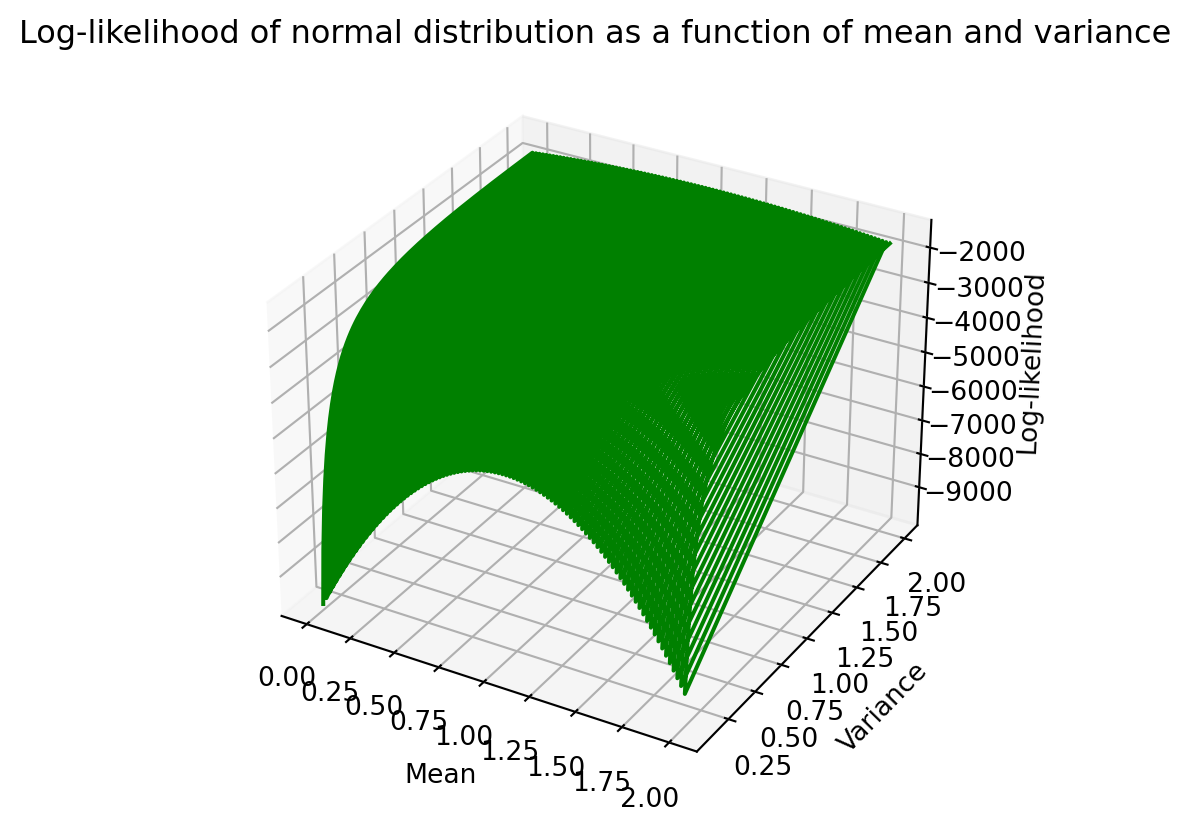
We can also visualize 3D plots in 2D using a contour plot. To do so, we can create a 100x100 grid (because we have 100 mean and variance values) and reshape Z’s shape to 100x100 so we have a value of log-likelihood for each point on the grid.
# Contour plot
fig,ax = plt.subplots()
X,Y,Z = log_likelihoods[:,0],log_likelihoods[:,1],log_likelihoods[:,2]
X,Y = np.meshgrid(np.unique(X),np.unique(Y))
Z = Z.reshape(X.shape)
plt.contourf(X,Y,Z)
plt.colorbar()
ax.set_title("Contour plot")
ax.set_xlabel("Mean")
ax.set_ylabel("Variance")
plt.show()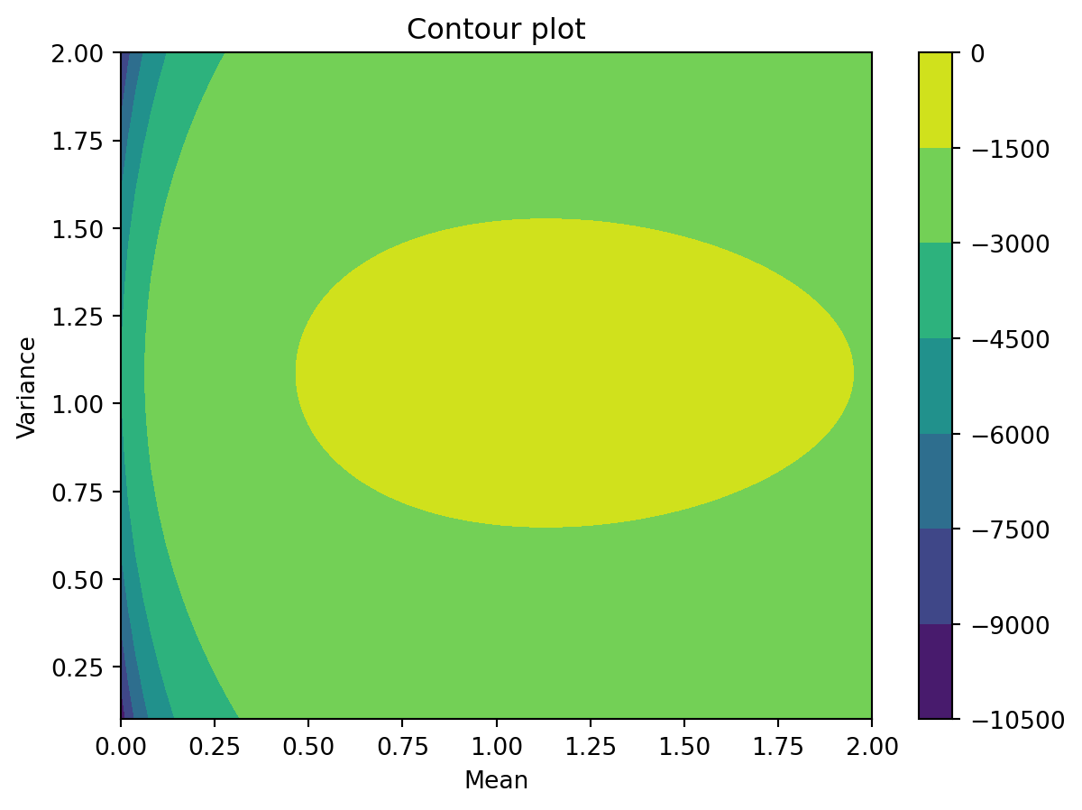
The values of mean and variance which will best fit the data will be those having the highest value of log-likelihood (Z-axis) and hence in the “yellow” region of the contour plot.